Tuesday, January 2, 2024

Testing RS41 current draw at different TX_POWER settings


Introduction

RS41ng on the RS-41 allows you to configure the output power via the  RADIO_SI4032_TX_POWER setting in the config.h file.  It allows values from 0-7.   I set out to determine how that setting impacts the RF output power as well as the current draw from the batteries during transmission.

Testing configuration


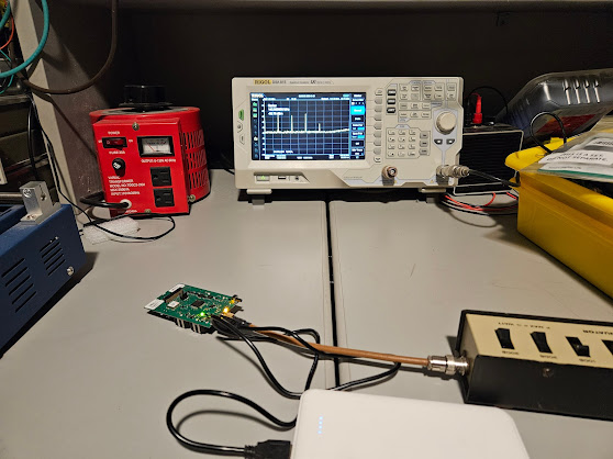
I configured a RS-41 with RS41ng.  The RS-41 has an SMA connector attached so that it could be wired through 19db of attenuators into a Spectrum Analyzer.  Power was provided by a bench power supply.  I varied the RADIO_SI4032_TX_POWER through various settings and measured both current draw and TX output power.  The basic setup as as follows:

Bench power supply voltage: 3.2 volts
Bench power supply max current: 0.650 amps


Frequency: 432.605mhz
Modulation: Horus Binary V2

Testing

For each test, I reprogrammed the RS-41 with a different RADIO_SI4032_TX_POWER setting and measured the output on the Spectrum Analyzer as well as the current draw on the bench power supply.

Example current draw when testing with the TX power set to 30:


Example Spectrum Analyzer result:


Results

 
RADIO_SI4032_TX_POWER DBM Current (ma)
Idle Consumption n/a
133
0 -4.5 172
1 -1.25
174
2 1.0
179
3 4.5
184
4 7.7
190
5
10.9
205
6 13.6
218
7
15.0
225

Conclusions

For airborne use,  14dbm (25mW) has been observed to be sufficient for line of site reception of Horus Binary using other trackers.  By setting RADIO_SI4032_TX_POWER set to 6 or 7, the desired output power is achieved. 


Saturday, December 30, 2023

Testing DFM17 Current draw at different TX_POWER settings

Introduction

RS41ng on the DFM17 allows you to configure the output power via the  RADIO_SI4063_TX_POWER setting in the config.h file.  It allows values from 0-127.   I set out to determine how that setting impacts the RF output power as well as the current draw from the batteries during transmission.

Testing configuration


I configured a DFM-17 with RS41ng.  The DFM-17 has an SMA connector attached so that it could be wired through 19db of attenuators into a Spectrum Analyzer.  Power was provided by a bench power supply.  I varied the RADIO_SI4063_TX_POWER through various settings and measured both current draw and TX output power.  The basic setup as as follows:

Bench power supply voltage: 7.5 volts
Bench power supply max current: 0.650 amps


Frequency: 432.605mhz
Modulation: Horus Binary V2

Testing

For each test, I reprogrammed the DFM-17 with a different RADIO_SI4063_TX_POWER setting and measured the output on the Spectrum Analyzer as well as the current draw on the bench power supply.

Example current draw when testing with the TX power set to 30:


Example Spectrum Analyzer result:


Results

 
RADIO_SI4063_TX_POWER DBM Current (ma)
Idle Consumption n/a
65
1 -12.0 76
12 3.0 90
25 9.0
107
30 10.4
112
45 14.0
128
50
14.7
132
75 17.8
151
100
18.8
162
127
19.2
182

Conclusions

For airborne use,  14dbm (25mW) has been observed to be sufficient for line of site reception of Horus Binary using other trackers.  By setting RADIO_SI4063_TX_POWER set to 45, the power consumption is about 70% of transmitting at full power.  The reduced power consuption would lead to longer battery life during flight, or on the ground during a HAB recovery.  


Wednesday, December 27, 2023

A little "science" on the DFM-17 running on 2m vs 70cm

The Experiment

I put on my lab coat, started boiling some test tubes, and made a few bwoo-hahaha noises tonight, as I did some science.  I attached an SMA connector to one of my DFM-17's so that I could run some controlled experiments of RS41ng on both 2m vs 70cm.  The intent was to verify whether the output RF filters on the DFM-17 are appropriate for transmitting beacons on the 2m band.

Modifying the DFM-17

I removed the stock antenna and added an SMA connector on the provided pads.  The board layout was standard, and an SMA connector in my parts bin fit just fine.


The test setup


I then cabled the DFM-17 through a pushbutton attenuator and added 40db of attenuation in the path to my Spectrum Analyzer (I didn't want to overdrive the input).  Note, the pushbutton attenuator I was using is built for 75 ohm, not 50 ohm.  This may impact some output power readings, but it should be consistent across frequencies, so while the output measured may not be exact, the relative powers and presence (or lack) of harmonic signals should be close enough for folk music and ham radio.


70cm Measurement

I then took a look at the spectrum when running at Horus Binary and APRS on 70cm.  I had the Spectrum Analyzer set to full scale (0-1500 mhz).  Note there were no harmonics in evidence at all.  The filters on the board seemed to do an admirable job of keeping it clean.  The SA showed -15 db.  Adding the 40db of attenuation, it's making about 25dbm of output.  Ish.


2m Measurement

I then re-flashed the code to beacon APRS at 144.390, and transmit Horus Binary at 145.600.  Note the harmonics generated.  The filtering on the board appears to be a low pass filter tuned to 70cm  So the harmonics below 400 mhz are coming through loud and clear.  There does seem to be some attenuation, as the signal on 144.390 is showing 10db weaker than the 70cm test).  The first and second harmonics have pretty strong relative output power, since they are presumably going through less attenuation as the frequencies increase.  There could be some variability in the output power of the Si4063 chip at different frequencies as well.  Note that the harmonic up in the 70cm frequency range is even stronger than the base signal at 2m, due to the vagaries of the filtering.


Conclusions

Running the DFM-17 below 70cm is going to transmit unwanted harmonics.  Though the overall output power is low, down in the 15dbm range, this would be generated by a balloon aloft, meaning the harmonics will be broadcast for pretty much line of sight across quite a significant radius.  I would advise against doing it unless you modify the filtering on the board.  The DFM-17 seems VERY nicely tuned for signals on 70cm, however.  I was quite pleased to see the results there.

Mike / KD2EAT


Sunday, February 16, 2020

Helical antenna for LMS6 radiosondes

Helical antenna for LMS6 radiosondes


The National Weather Service in Buffalo, NY launches two weather sondes per day.  They presently use Lockheed Martin LMS6 Radiosondes running at 1680(ish) MHZ and intend to continue running the until sometime in 2020.   Since I'd like to track them, I wanted to build an optimized antenna system.

Antenna Design


The LMS6 uses a Left Hand Circularly Polarized (LHCP) patch antenna.  (Note: I read this somewhere, but I'll be darned if I can now find the information.  If you happen to have documentation of that fact, I'd love to have it!)  Therefore, for best range, I opted to build an LHCP antenna for my receive station.  Looking online, I quickly found an online calculator and came up with the following model.

  • Assumed Velocity Factor: 100%
    • Frequency: 1680 mhz
    • Wavelength: 178.6 mm
    • Diameter: 58.9 mm
    • Spacing (.25 wave): 44.6 mm

Build

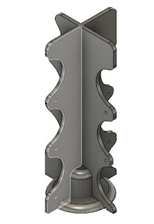
Using these characteristics, I used Fusion 360 to design a "holder" for the spiral of wire I would use for the antenna.  I configured a 1/4" x 20 threaded mounting hole in the bottom so that it could be screwed down to a reflector, and the same threaded rod could be used on the bottom to secure a 1/4" x 20 coupling nut.  That nut could be used to mount the reflector on a standard camera tripod.

The 3D Design looked like this:


I used bare 16ga wire for the element.  I pre-wrapped it around a 2" mailer tube to get the shape right, and then fed it through the structure.  I bought a lid for a pot at a local reuse store for $1 to use as my reflector.   I installed a bulkhead SMA adapter on the lid, near the base of the spiral.  The result looked like this:


Testing


Unfortunately, the online model does not account for velocity factor.  When I did an SWR measurement on the antenna, it was out of tune in the frequency of interest.  I did about 1/2 dozen prints, and resolved that 95% velocity factor was the ideal for this design.

  • Velocity Factor: 95%
    • Frequency: 1680 mhz
    • Wavelength: 169.6 mm
    • Diameter: 54.0 mm
    • Spacing (.25 wave): 42.4 mm

With those parameters, I ran a VSWR plot, and it looked great!  The plot is centered at 1680 mhz, and the two markers are at the approximate end points of the range of frequencies we might see from an LMS6 sonde running at 1680 mhz.


In use


I took the antenna out and compared it to a 1/4 wave dipole antenna (which also has very good VSWR) and the results were significantly better.  I was running two Raspberry Pi's in my vehicle, running radiosonde_auto_rx software with identical SDRs and preamps.  The helical began receiving the sonde about 30 miles (48 km) distant.  My dipole running, simultaneously, did not beg receiving the sonde until about 10 miles out.  That's only one data point, so far, but I'm pleased by the initial findings.

Here's an image of my chase vehicle, with a dipole duct-taped to the roof rack, and the helical set up on a tripod beside the car.


Further testing


I'd like to gather more side by side comparisons of the performance of these antennas during radiosonde hunts.  That will be greatly facilitated if one of them (finally!) lands somewhere that I can retrieve it.  My area of Central New York State features an awful lot of tall trees!  Once I have one in hand, I can use it for real-world signals in a more controlled laboratory environment.


Sunday, December 29, 2019

radiosonde_auto_rx addition - OLED display

The problem with auto_rx on a "headless" Raspberry Pi


So, the Project Horus "radiosonde_auto_rx" package is a wonderful bit of software that one can run on a Raspberry Pi to automatically detect and upload radiosonde data to the CUFS Predictor site.  They've also front-ended that site with one specifically for weathersondes at https://tracker.sondehub.org.

Unfortunately, it's the kind of thing I'd prefer to run "headless" and save the space and expense of keeping a keyboard, monitor and mouse attached to my Raspberry Pi.  I would also like to be able to use it in a mobile application, rather than the Project Horus chasemapper software.  While Chasemapper looks like great software, I presently run HAB chases with Windows APRSISCE32 software.  I run a windows laptop in my chase vehicle, and expect to continue doing so. Therefore, when running with auto_rx, I'd like to keep the mobile footprint of my weather sonde gear minimal and use my Windows laptop.  Therefore, I decided to add an OLED display to the, otherwise headless, Raspberry Pi.

The OLED


I picked up some very cheap (like under $2 each) 0.96" monochrome 128x64 OLED displays from Banggood.  I won't post a link as they seem to come and go with inventory.  The particular model that I got actually has the first 16 rows of pixels in yellow, and the rest in blue.  That actually works out well for my plans, as I'd like to use the top rows for static data, and the lower rows for a scrolling text area with incoming telemetry.


The OLED is an I2C device.  It easily plugs into a Raspberry Pi on pins 1, 3, 5, 6. 

Python Library


It was harder than I expected to find a good library for the OLED in the Raspberry Pi.  Several were expecting Python 2.  Others that I expected to work had dependency problems.  Adafruit was suggesting using their Circuitpython libraries, but I couldn't get them to work.  I ended up downloading Adafruit's legacy Adafruit_SSD1306 library and using that.

Todo: I should really download a contemporary library and get this code working with it.

Interfacing with auto_rx


The next decision was about how to interface with auto_rx as seamlessly as possible.  Project Horus made that very easy by providing the data I wanted via UDP broadcast.  By setting "payoad_summary_enabled" to "True" in the "station.cfg" file of auto_rx, they enable broadcasts.  While intended for use with their Chasemapper app, there's no reason we can't piggy-back on that functionality to get the payload data out separately with no mods at all to the stock auto_rx code.

The basic script

My "runoled.py" script is very simple.  It's basically doing this:

    Initialize OLED
    Initialize UDP Listener
    while (1) 
       update_OLED
          Update first two lines with IP addr and SSID
          Print out the next 6 lines of scrolling text.
       sleep(1)


The real magic comes in when a new UDP packet comes in.  When it does, the interrupt routine updates the 6 lines of rolling text for the OLED display, preparing it for the next update in the main program loop..


def handle_payload_summary(packet)
    ...
    oled_line1 = oled_line2
    oled_line2 = oled_line3
    oled_line3 = oled_line4
    oled_line4 = oled_line5
    oled_line5 = oled_line6
    oled_line6 = _time + ' ' + str(_alt)

This just rolls the lines from bottom to top, and puts the latest packet data (time and altitude) on the bottom. As additional packets come in, we'll scroll the oldest up, and then off.

How it looks in action


Here's an example of how the OLED works on my Pi.  I have the Pi installed in a cheap clear case.  I drilled a hole in it to mount the OLED, and poke the riser pins through the cover.  They're wired to the GPIO riser inside the case.  It's just taped together for now.  If I get fancy, I might install some screws.  The data in the display is just fabricated times and altitudes that I sent to the script via a test program that uses the same library calls that auto_rx uses.


Network display and Wifi setup


I configure multiple SSID's on my auto_rx Raspberry Pi.  When it's in my home, it joins to my home network.  When I'm out in my car, I have it join my cell phone's tether SSID.  I have the first two lines of the OLED set up so that I can see the IP address of the Pi, and also the SSID that it has joined.  This gives me visual confirmation that the Pi is up and running on the network.

I rum a proxy ssh solution on my Pi, so that I can SSH into it, even when on my cell phone tether.

Automated startup


I have the script set up to run out of /etc/rc.local so that it starts at boot time.  I can monitor the first two lines of the OLED to confirm the Pi is on the network, and then when packets start arriving, the timestamp and altitude begin scrolling from the bottom.  

From /etc/rc.local:
/bin/su --login pi -c /home/pi/src/oled/runoled.py > /tmp/runoled.log 2>&1 &


The full source of runoled.py


Shipped by weight not volume.  Some settling may have occurred during shipping.  Actual color may vary from the packaging.   If you experience any unpleasant side effects, discontinue use immediately.


#!/usr/bin/env python
#
#   radiosonde_auto_rx - 'Horus UDP' Receiver Example
#
#   Copyright (C) 2019  Mark Jessop <vk5qi@rfhead.net>
#   Released under GNU GPL v3 or later
#
#   This code provides an example of how the Horus UDP packets emitted by auto_rx can be received
#   using Python. Horus UDP packets are simply JSON blobs, which all must at the very least contain a 'type' field, which
#   (as the name suggests) indicates the packet type. auto_rx emits packets of type 'PAYLOAD_SUMMARY', which contain a summary
#   of payload telemetry information (latitude, longitude, altitude, callsign, etc...)
#
#   Output of Horus UDP packets is enabled using the payload_summary_enabled option in the config file.
#   See here for information: https://github.com/projecthorus/radiosonde_auto_rx/wiki/Configuration-Settings#payload-summary-output
#   By default these messages are emitted on port 55672, but this can be changed.
#
#   In this example I use a UDPListener object (ripped from the horus_utils repository) to listen for UDP packets in a thread,
#   and pass packets that have a 'PAYLOAD_SUMMARY' type field to a callback, where they are printed.
#

import datetime
import json
import pprint
import socket
import time
import traceback
from threading import Thread

import Adafruit_GPIO.SPI as SPI
import Adafruit_SSD1306

from PIL import Image
from PIL import ImageDraw
from PIL import ImageFont

import subprocess

oled_line1 = ""
oled_line2 = ""
oled_line3 = ""
oled_line4 = ""
oled_line5 = ""
oled_line6 = ""


class UDPListener(object):
    ''' UDP Broadcast Packet Listener
    Listens for Horus UDP broadcast packets, and passes them onto a callback function
    '''

    def __init__(self,
        callback=None,
        summary_callback = None,
        gps_callback = None,
        port=55673):

        self.udp_port = port
        self.callback = callback

        self.listener_thread = None
        self.s = None
        self.udp_listener_running = False


    def handle_udp_packet(self, packet):
        ''' Process a received UDP packet '''
        try:
            # The packet should contain a JSON blob. Attempt to parse it in.
            print "Packet received"
            packet_dict = json.loads(packet)

            # This example only passes on Payload Summary packets, which have the type 'PAYLOAD_SUMMARY'
            # For more information on other packet types that are used, refer to:
            # https://github.com/projecthorus/horus_utils/wiki/5.-UDP-Broadcast-Messages
            if packet_dict['type'] == 'PAYLOAD_SUMMARY':
                if self.callback is not None:
                    self.callback(packet_dict)

        except Exception as e:
            print("Could not parse packet: %s" % str(e))
            traceback.print_exc()


    def udp_rx_thread(self):
        ''' Listen for Broadcast UDP packets '''

        self.s = socket.socket(socket.AF_INET,socket.SOCK_DGRAM)
        self.s.settimeout(1)
        self.s.setsockopt(socket.SOL_SOCKET, socket.SO_REUSEADDR, 1)
        try:
            self.s.setsockopt(socket.SOL_SOCKET, socket.SO_REUSEPORT, 1)
        except:
            pass
        self.s.bind(('',self.udp_port))
        print("Started UDP Listener Thread on port %d." % self.udp_port)
        self.udp_listener_running = True

        # Loop and continue to receive UDP packets.
        while self.udp_listener_running:
            try:
                # Block until a packet is received, or we timeout.
                m = self.s.recvfrom(1024)
            except socket.timeout:
                # Timeout! Continue around the loop...
                m = None
            except:
                # If we don't timeout then something has broken with the socket.
                traceback.print_exc()

            # If we hae packet data, handle it.
            if m != None:
                self.handle_udp_packet(m[0])

        print("Closing UDP Listener")
        self.s.close()


    def start(self):
        if self.listener_thread is None:
            self.listener_thread = Thread(target=self.udp_rx_thread)
            self.listener_thread.start()


    def close(self):
        self.udp_listener_running = False
        self.listener_thread.join()


def handle_payload_summary(packet):
    global oled_line1
    global oled_line2
    global oled_line3
    global oled_line4
    global oled_line5
    global oled_line6

    ''' Handle a 'Payload Summary' UDP broadcast message, supplied as a dict. '''

    # Pretty-print the contents of the supplied dictionary.
    pprint.pprint(packet)

    # Extract the fields that should always be provided.
    _callsign = packet['callsign']
    _lat = packet['latitude']
    _lon = packet['longitude']
    _alt = packet['altitude']
    _time = packet['time']

    # The comment field isn't always provided.
    if 'comment' in packet:
        _comment = packet['comment']
    else:
        _comment = "No Comment Provided"

    # Do nothing with these values in this example...
    oled_line1 = oled_line2
    oled_line2 = oled_line3
    oled_line3 = oled_line4
    oled_line4 = oled_line5
    oled_line5 = oled_line6
    oled_line6 = _time + ' ' + str(_alt)


if __name__ == '__main__':
    # Raspberry Pi pin configuration:
    RST = None     # on the PiOLED this pin isnt used
    # Note the following are only used with SPI:
    DC = 23
    SPI_PORT = 0
    SPI_DEVICE = 0
    # 128x64 display with hardware I2C:
    disp = Adafruit_SSD1306.SSD1306_128_64(rst=RST)
    # Initialize library.
    disp.begin()

    # Clear display.
    disp.clear()
    disp.display()

    # Create blank image for drawing.
    # Make sure to create image with mode '1' for 1-bit color.
    width = disp.width
    height = disp.height
    image = Image.new('1', (width, height))

    # Get drawing object to draw on image.
    draw = ImageDraw.Draw(image)

    # Draw a black filled box to clear the image.
    draw.rectangle((0,0,width,height), outline=0, fill=0)

    # Draw some shapes.
    # First define some constants to allow easy resizing of shapes.
    padding = -2
    top = padding
    bottom = height-padding
    # Move left to right keeping track of the current x position for drawing shapes.
    x = 0

    # Load default font.
    font = ImageFont.load_default()
    draw.text((x, top),       "Booting",  font=font, fill=255)
    # Display image.
    disp.image(image)
    disp.display()
################################################################################################
    # Instantiate the UDP listener.
    udp_rx = UDPListener(
        port=55673,
        callback = handle_payload_summary
        )
    # and start it
    udp_rx.start()

    # From here, everything happens in the callback function above.
    try:
        while True:

            # Draw a black filled box to clear the image.
            draw.rectangle((0,0,width,height), outline=0, fill=0)

            # Shell scripts for system monitoring from here : https://unix.stackexchange.com/questions/119126/command-to-display-memory-usage-disk-usage-and-cpu-load
            cmd = "hostname -I | cut -d\' \' -f1"
            IP = subprocess.check_output(cmd, shell = True )

            cmd = "/sbin/iwgetid"
            try:
               SSID = subprocess.check_output(cmd, shell = True )
            except:
               SSID = '"None"'
            SSID = SSID[SSID.find('"')+1:SSID.rfind('"')]

            # Write two lines of text.

            draw.text((x, top),       "IP: " + str(IP),  font=font, fill=255)
            draw.text((x, top+8),     "SSID: " + str(SSID[0:10]), font=font, fill=255)
            draw.text((x, top+16),    oled_line1,  font=font, fill=255)
            draw.text((x, top+24),    oled_line2,  font=font, fill=255)
            draw.text((x, top+32),    oled_line3,  font=font, fill=255)
            draw.text((x, top+40),    oled_line4,  font=font, fill=255)
            draw.text((x, top+48),    oled_line5,  font=font, fill=255)
            draw.text((x, top+56),    oled_line6,  font=font, fill=255)

            # Display image.
            disp.image(image)
            disp.display()

            time.sleep(1)
    # Catch CTRL+C nicely.
    except KeyboardInterrupt:
        # Close UDP listener.
        udp_rx.close()
        # Draw a black filled box to clear the image.
        draw.rectangle((0,0,width,height), outline=0, fill=0)
        # Display image.
        disp.image(image)
        disp.display()
        print("Closing.")


Full source of "send.py"


This program sends UDP packets to the OLED daemon, so that I can test it without waiting for a balloon to come by.  It uses the same subroutine calls that auto_rx uses.  Note, this script isn't pretty.  It was just hacked at until it worked well enough to test the OLED.  I'm not really familiar with the time and datetime libraries or I'm sure I could have done something prettier.

Note, you'll need to set your PYTHONPATH to point into the autorx directories to use this.  Ex:
    $ export PYTHONPATH=/home/pi/src/projecthorus/radiosonde_auto_rx/auto_rx:$PYTHONPATH

Here's the code:

import time
import datetime
from autorx.ozimux import OziUploader
from time import gmtime, localtime

dt = datetime.datetime(2019, 12, 29, 20, 03, 04, 79043)
gmt = gmtime()

ozimux = OziUploader(
    ozimux_port = None,
    payload_summary_port = 55673,
    update_rate = 5,
    station='KD2EAT')


packet = {
    'frame' : '1',
    'id' : '1',
    'datetime' : gmt,
    'lat' : 42.4417,
    'lon' : -76.4985,
    'alt' : 22345,
    'temp': 32,
    'type' : 'PAYLOAD_SUMMARY',
    'freq': '1678',
    'freq_float': 1678.0,
    'datetime_dt' : dt,
    }

_short_time = packet['datetime_dt'].strftime("%H:%M:%S")
ozimux.add(  packet )
print "Sent. sleeping 10 to avoid race condition where we shut down before sending the packet."
time.sleep(10)

ozimux.close()
print "Closed"


Weather sonde automated prediction

Weather Sonde automated prediction


So, I've gotten the bug to chase weather balloons.  The balloons in my region are launched by the National Weather Service from a location adjoining the airport in Buffalo, New York.   Only a small percentage of the balloons make it southeast enough to be within reasonable chase distance from my home near Ithaca, New York, 110 air miles away.  I ran manual predictions every day, to see how the balloons might progress, but that got tedious.  I decided some automation was in order.

CUFS Prediction Software

To begin, I picked up the CUFS Prediction Wrapper for python.  It provided tools to download the latest NWS prediction data as well as tools to run predictions.  I run a Raspberry Pi at home, so I set up cron jobs to load the data each morning, and to run predictions for the next 7 days.

Downloading Wind Data

I set up a cron job to download the wind data at 3am each day:

0 3 * * * /home/mqh1/bin/wind_grabber.sh > /home/mqh1/balloons/cusf/logs/windgrabber.log 2>& 1

The contents of the "wind_grabber.sh' script are as follows:

python \
/home/mqh1/balloons/cusf/cusf_predictor_wrapper/apps/get_wind_data.py \
--lat=42 --lon=-77 --latdelta=2 --londelta=4 -f 180 \
-m 0p25_1hr -o /tmp/gfs/

The lat/long as well as latedelta/londelta parameters are sufficient to include most of the likely flight locations of a weather balloon out of Buffalo.  I cache the results in /tmp/gfs on the pi.  "-f 180" is looking for the next 180 hours of predictions (7 1/2 days).

The result is that I have current wind data automatically downloaded on a daily basis that should cover the areas of interest for any NWS flights.  Since I do my own High Altitude Balloon launches, as well as pico flights, I don't feel too guilty about downloading this data daily.

Todo: I'd like to find out when the NWS uploads the data, and tune my download and daily prediction schedule to use the latest data.

Running predictions


Typical flights

I was curious what the best parameters would be to choose for ascent rate / descent rate / and burst altitude for the NWS balloon.  Fortunately, two of the three are provided on a regular basis by the NWS.  They have an index with the codes for all the launch locations. I was able to download a big file with all of the flight data from the last two years of flights.  I stuck it in a spreadsheet, and did some number crunching.  I had to eliminate a few flights that were clearly outliers.  They had really screwy ascent rates or burst altitudes compared to the rest.  I removed the anomalies that had glaring differences, and ran averages on the remainder.  I got the following averages.

Average burst altitude: 31,420 meters
Average ascent rate: 5.28 m/sec

Unfortunately, the NWS doesn't log the descent data, so I don't have a good measure of the average descent rate of the sondes.  Based on conversations with folks who do this, it seems like most people go with 5m/s.  It can vary widely however.

Todo: If I get a fully automated station running, I'd like to get better data about descent rates and decide how to handle it.  I might use an average, or I might do predictions on each end of the range.

Automated predictions

The CUSF software makes it really easy to run predictions.  I run them after I download the GFS data.  I haven't measured the typical download rate yet, so for now, I run them 90 minutes after the  wind data download.

30 4 * * * /home/mqh1/bin/sonde_predict.py > /home/mqh1/balloons/cusf/logs/sonde_predict.log 2>& 1

The prediction script is a bit more complicated than the download script.  I started from the sonde_predict.py script provided by the CUSF wrapper and made three principal mods. 

  1. Determining which predictions are coming in "near' Ithaac
  2. Generating two separate KML files.  One for "nearby" and one for "all" predictions.
  3. Emailing results.

Determining nearby predictions

After the prediction runs, I take the final landing coordinates and determine whether they are "nearby" Ithaca.  I do this with a Point in Polygon (PIP) algorithm.

 I used Google Earth to draw a bounding box covering an area around Ithaca in which I was willing to search for balloons (Add / Polygon).  I then exported the polygon to a KML (right-click, Save Place As),  I was then able to grab the coordinates from the KML file, and just copy/paste them to create an array in the code.  Note, I had edit the data to reverse the lat/long coming out of the KML file to make them more friendly.  In retrospect, I could have left them reversed, and just reversed the order in the code below.  Still, I think this is more "human friendly" to see them in the typical order.

# Coordinate around Ithaca (larger grid)
nearby_coords = [
   (42.5894692373013, -77.13750089643533),
   (42.13873798563936, -77.11683620792473),
   (42.1355764571338, -75.91998110781731),
   (42.62563890419801, -75.89559117314741)
   ]


The coords of the prediction of the payload are in the script in the flight_path[] array, so we grab the last position.

        finalcoords = flight_path[-1]
        latlong = (finalcoords[1], finalcoords[2])
        landingsite = Point(latlong)

Then we can determine whether it's in the "nearby_coords" polygon we've established:

        if landingsite.within(nearby_poly):

Creating a second KML file


If we're within the "nearby_poly", I add the KML plot to a separate list.  I modified the provided script to generate two KML files.  One for "all' predictions, and one for "nearby" predictions.   I write both of the predictions into an HTML directory for the web server I run on the Pi.  That makes it trivial to download them to my laptop to inspect them with Google Earth.

Emailing results

Finally, I modified the prediction script to generate an email summarizing the number of nearby predictions, and containing HTML links to both the nearby and full KML files.  Each morning, I receive an email that tells me if I have nearby predictions.  If I do, I can click the link to see the predictions for the coming week that land near Ithaca.


In the image below, I highlighted the bounding box for my "nearby" predictions.


Todo: I'd like to find a way to provide a link into google maps which will show the 2D representation of the prediction by just clicking a link, rather than having to download a KML file and launch Google Earth.

Sample Code


Disclaimers: Shipped by weight not volume.  Some settling may occur during shipping.  Not actual size.  Consult your computer professional before running.  If this code causes and erection lasting more than 4 hours, consult a physician.. no, seriously!

#!/usr/bin/env python
#
#   Project Horus
#   CUSF Standalone Predictor Python Wrapper
#       Radiosonde Launch Predictor
#   Copyright 2017 Mark Jessop <vk5qi@rfhead.net>
#
#       In this example we run predictions for a radiosonde launch from Adelaide Airport
#       for every launch for the next 7 days, and write the tracks out to a KML file.
#
#       For this script to work correctly, we need a weeks worth of GFS data available within the gfs directory.
#       This can be gathered using get_wind_data.py (or scripted with wind_grabber.sh), using :
#           python get_wind_data.py --lat=-33 --lon=139 --latdelta=10 --londelta=10 -f 168 -m 0p25_1hr -o gfs
#       with lat/lon parameters chaged as appropriate.
#
# Mods to this script written by Mike Hojnowski / KD2EAT.  It is provided for informational purposes.  It will
# not run in a generic environment without modification.  In particular, look for the email addresses and for
# the home directories sprinkled in paths all over.
#

import smtplib
import time
import fastkml
import datetime
from dateutil.parser import parse
from cusfpredict.predict import Predictor
from pygeoif.geometry import Point, LineString
from cusfpredict.utils import *
from shapely.geometry import Point, Polygon

#Email Variables
SMTP_SERVER = 'smtp.gmail.com' #Email Server (don't change!)
SMTP_PORT = 587 #Server Port (don't change!)
GMAIL_USERNAME = 'somebody@gmail.com' #change this to match your gmail account
GMAIL_PASSWORD = 'ImDumbButNotTHATDumb'  #change this to match your gmail password
SENDTO = 'ThisCouldBeYou@gmail.com'     #change to the recipient of the emails

## Coordinate around Ithaca (smaller grid)
#nearby_coords = [
#   (42.44387782645627, -77.01612142816262),
#   (42.2569086411454,-76.99969683890008),
#   (42.3432446683892, -76.17009222210787),
#   (42.57580936472674, -76.28671583838107),
#   ]
#

# Coordinate around Ithaca (larger grid)
nearby_coords = [
   (42.5894692373013, -77.13750089643533),
   (42.13873798563936, -77.11683620792473),
   (42.1355764571338, -75.91998110781731),
   (42.62563890419801, -75.89559117314741)
   ]

nearby_poly = Polygon(nearby_coords)

# BIG polygon for testing. No predictions were near Ithaca the day I was coding, so I made a bigger polygon.
huge_coords = [
   (43.44387782645627, -78.01612142816262),
   (41.2569086411454,-78.99969683890008),
   (41.3432446683892, -75.17009222210787),
   (43.57580936472674, -75.28671583838107),
   ]

# Just substitude "huge_poly" for "nearby_poly" in the code below, if you need to test during unfavorable predictions.
huge_poly = Polygon(huge_coords)


# Predictor Parameters
PRED_BINARY = "/home/mqh1/balloons/cusf/cusf_predictor_wrapper/apps/pred"
GFS_PATH = "/tmp/gfs"

NEARBY_OUTPUT_FILE = "/home/mqh1/public_html/nearby_predictions.kml"
ALL_OUTPUT_FILE = "/home/mqh1/public_html/all_predictions.kml"

# Launch Parameters - Update as appropriate for your launch site
# Launch parameters based on NWS data from 01/01/2018 - 12/22/2019 averages
LAUNCH_LAT = 42.9414
LAUNCH_LON = -78.7193
LAUNCH_ALT = (218+500)/2.0;             # Barometric and GPS varied.  I took the average.
ASCENT_RATE = 5.26
DESCENT_RATE = 5.0
BURST_ALT = 31420

# Set the launch time to the current UTC day, but set the hours to the 12Z sonde
current_day = datetime.datetime.utcnow()
LAUNCH_TIME = datetime.datetime(current_day.year, current_day.month, current_day.day, 11, 15)


# Parameter Variations
# These can all be left at zero, or you can add a range of delta values
launch_time_variations = range(0,168,12) # Every 12 hours from now until 7 days time.

# A list to store prediction results
nearby_predictions = []
all_predictions = []
nearby = 0

# Create the predictor object.
pred = Predictor(bin_path=PRED_BINARY, gfs_path=GFS_PATH)

# Iterate through the range of launch times set above
for _delta_time in launch_time_variations:

        # Calculate the launch time for the current prediction.
        _launch_time = LAUNCH_TIME + datetime.timedelta(seconds=_delta_time*3600)

        print ('Running prediction for ' + str(_launch_time))
        # Run the prediction
        flight_path = pred.predict(
                launch_lat=LAUNCH_LAT,
                launch_lon=LAUNCH_LON,
                launch_alt=LAUNCH_ALT,
                ascent_rate=ASCENT_RATE,
                descent_rate=DESCENT_RATE,
                burst_alt=BURST_ALT,
                launch_time=_launch_time)

        # If we only get a single entry in the output array, it means we don't have any wind data for this time
        # Continue on to the next launch time.
        if len(flight_path) == 1:
                continue

        #print(flight_path[-1])
        coords = flight_path[-1]
        latlong = (coords[1], coords[2])
        #print latlong
        landingsite = Point(latlong)
        #print landingsite.within(nearby_poly)
        #print landingsite.within(huge_poly)

        # Generate a descriptive comment for the track and placemark.
        pred_time_string = _launch_time.strftime("%Y%m%d-%H%M")
        pred_comment = "%s %.1f/%.1f/%.1f" % (pred_time_string, ASCENT_RATE, BURST_ALT, DESCENT_RATE)

        # Add the track and placemark to our list of predictions
        all_predictions.append(flight_path_to_geometry(flight_path, comment=pred_comment))
        all_predictions.append(flight_path_landing_placemark(flight_path, comment=pred_comment))

        if landingsite.within(nearby_poly):
                # If nearby, add the placemark to our nearby predictions list
                nearby_predictions.append(flight_path_to_geometry(flight_path, comment=pred_comment))
                nearby_predictions.append(flight_path_landing_placemark(flight_path, comment=pred_comment))
                print("Prediction Succeeds: %s" % pred_comment)
                nearby += 1

# Write out the prediction data to the KML file
kml_comment = "Sonde Predictions - %s" % gfs_model_age()
write_flight_path_kml(all_predictions, filename=ALL_OUTPUT_FILE, comment=kml_comment)
write_flight_path_kml(nearby_predictions, filename=NEARBY_OUTPUT_FILE, comment=kml_comment)

###################
# Email portion

class Emailer:
    def sendmail(self, recipient, subject, content):

        #Create Headers
        headers = ["From: " + GMAIL_USERNAME, "Subject: " + subject, "To: " + recipient,
                   "MIME-Version: 1.0", "Content-Type: text/html"]
        headers = "\r\n".join(headers)

        #Connect to Gmail Server
        session = smtplib.SMTP(SMTP_SERVER, SMTP_PORT)
        session.ehlo()
        session.starttls()
        session.ehlo()

        #Login to Gmail
        session.login(GMAIL_USERNAME, GMAIL_PASSWORD)

        #Send Email & Exit
        session.sendmail(GMAIL_USERNAME, recipient, headers + "\r\n\r\n" + content)
        session.quit

sender = Emailer()

sendTo = SENDTO
emailSubject = "Sonde predictions nearby: " + str(nearby)
emailContent = str(nearby) + ' predictions have been detected near Ithaca.<br><br>'  +\
   '\nNearby Predictions: <a href=http://thehojos.com/~mqh1/nearby_predictions.kml>http://thehojos.com/~mqh1/nearby_predictions.kml</a><br><br>' +\
   '\nAll Predictions: <a href=http://thehojos.com/~mqh1/all_predictions.kml>http://thehojos.com/~mqh1/all_predictions.kml</a>'

sender.sendmail(sendTo, emailSubject, emailContent)
print("Email Sent")